Mode connectivity
The old picture of the loss surface as many isolated basins, one per initialization, has not held up. Freeman and Bruna [6] suggested early on that low-loss level sets stay connected. Garipov et al. [1] and Draxler et al. [2] then made it concrete: two independently trained models can be joined by a smooth low-loss path. The minima are not isolated points; they are reachable from each other through a connected high-dimensional region.
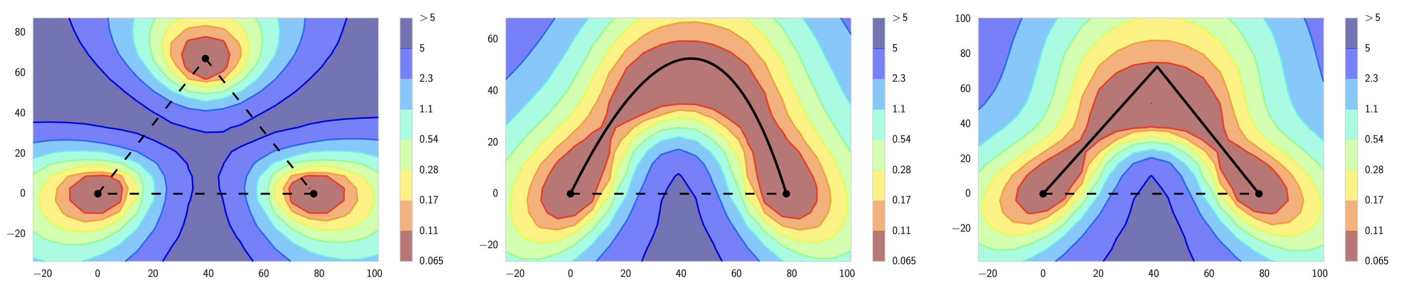
The experiment is direct. Train two models \(\theta_1\) and \(\theta_2\) to low loss, and interpolate linearly between them to define a one-parameter family \[\theta(\alpha) = (1-\alpha)\,\theta_1 + \alpha\,\theta_2\] for \(\alpha \in [0,1]\). The straight segment usually crosses a high-loss barrier \[B = \max_{\alpha \in [0,1]} L(\theta(\alpha)) - \tfrac{1}{2}\big(L(\theta_1) + L(\theta_2)\big).\] In other words, the loss jumps up substantially as soon as one steps off either endpoint, and the peak in the middle is typically far above either endpoint loss. Garipov and Draxler's contribution was to show that this barrier exists only along the straight line: if you allow curved paths, you can connect \(\theta_1\) and \(\theta_2\) with a path that stays at low loss throughout. The endpoints are not separated by an insurmountable barrier; the straight line is just the wrong path through parameter space.
Curves before lines
The first demonstrations of mode connectivity used non-linear paths. Garipov et al. parametrized the path as polygonal chains and Bézier curves; Draxler et al. used continuous non-linear paths produced by the Nudged Elastic Band method. Both findings weakened the previous picture in which SGD ends up in sharply-separated basins: if a low-loss path exists between two trained models, the connected low-loss region they both lie in is substantially larger than what a local Hessian analysis at either endpoint would suggest.
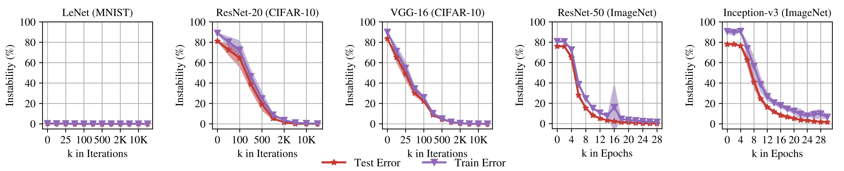
Linear mode connectivity is strictly stronger than the curve-based version: it asks the loss to stay low along the straight segment between two minima, not along an arbitrary path. For independently-trained networks from distinct initializations this typically fails. The linearly connected case is essentially confined to one setup. Frankle, Dziugaite, Roy, and Carbin [3] formalized it as "spawning": train a model \(\theta_0\), fork two copies after \(k\) steps using different SGD noise, and train each to convergence. Once \(k\) crosses a stability threshold (around 1000-2000 iterations on standard CIFAR networks, and a few percent of training on ImageNet), the two descendants end up linearly connected. They argue this is exactly the lottery-ticket basin: the connected region is the one that the matching sparse sub-network corresponds to, so linear-mode-connectivity becomes a practical test for whether two runs landed in the same effective basin and can therefore be merged without loss.
The permutation turn
Entezari et al. [4] reframed the geometry. Neural networks have permutation symmetries: swapping units in a hidden layer and unswapping them in the next layer leaves the function unchanged. Two models that look far apart in raw parameter coordinates might just be using different unit orderings of the same function. Quotient by those permutations and many independently trained models turn out to be connected by a simple low-loss curve.
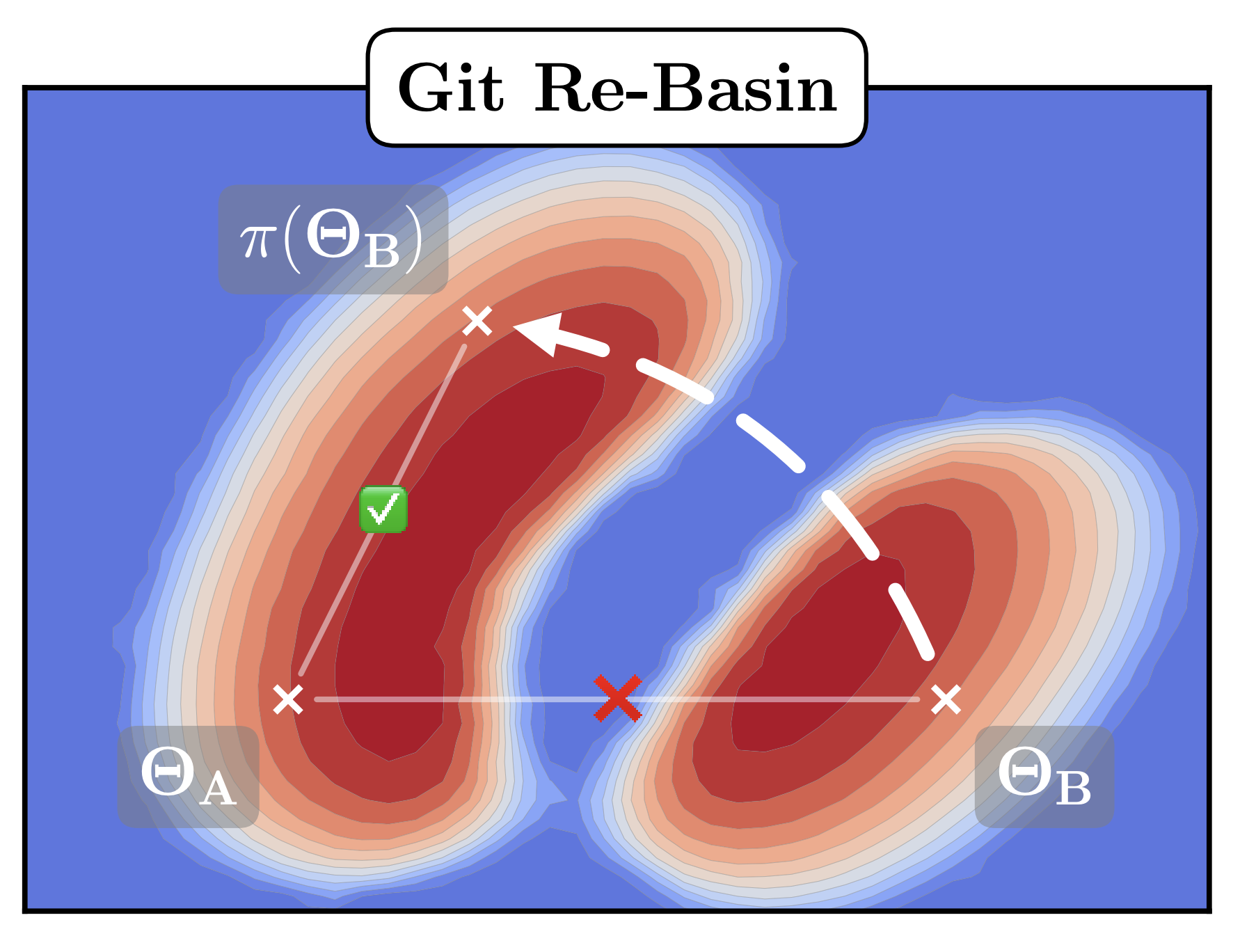
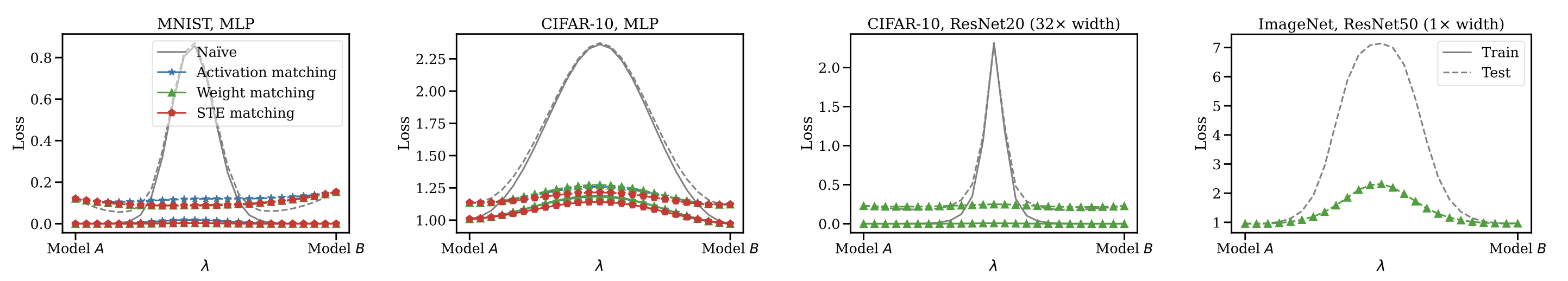
Git Re-Basin turns the idea into a concrete algorithm. Given two trained models $\theta_1, \theta_2$ with hidden-layer widths $\{n_\ell\}$, it searches over permutation matrices $P_\ell \in S_{n_\ell}$ for the alignment that minimizes $\lVert \theta_1 - P \cdot \theta_2 \rVert$ under a weights or activations metric, then checks whether the aligned models can be merged in weight space. Singh and Jaggi give an optimal-transport version of the same idea: a soft assignment between units that reduces to permutation matching when the widths agree, and that handles mismatched widths when they don't. Neither paper proves that all minima sit in one basin, but together they make a strong empirical case that raw parameter-space interpolation overstates the separation. A meaningful fraction of the apparent barrier is just a bad coordinate system.
Say you train Model A.
— Samuel "curry-howard fanboi" Ainsworth (@SamuelAinsworth) September 13, 2022
Independently, your friend trains Model B, possibly on different data.
With Git Re-Basin, you can merge models A+B in weight space at _no cost to the loss_
Empirical evidence ties together alignment and merging
Tatro et al. [7] showed empirically that aligning models before fitting a connecting curve produces shorter curves with lower loss along them, which is the consistency check the permutation story predicts: correcting for symmetries should give a simpler geometry than the raw view. Benton et al. [8] extended this beyond curves to higher-dimensional simplexes of solutions: once symmetries are corrected, low-loss volumes contain many independently trained checkpoints.
Practical applications
Model merging is what gets built on top. SWA averages late-training checkpoints and works because the trajectory it averages over stays inside one connected low-loss region. Model Soups average independently fine-tuned models from a shared pretraining initialization, which puts every fine-tune inside the same connected component and close to the others. Git Re-Basin generalizes this further by aligning unit permutations so models with no shared initialization can be merged at all. Across architectures, weight space behaves like a workspace where related models can be moved between while preserving function — once symmetries and shared training histories have been accounted for.
It does not explain generalization. A connected low-training-loss region can contain many bad predictors on held-out data, and showing that two solutions are connected says nothing about how either performs on unseen examples. It also does not guarantee that every architecture, dataset, or training recipe lives in a single basin; the broader single-basin claims have counter-examples. I read "one wide basin" as rhetorically appealing but over-reaching the evidence. The established claim is weaker: solutions reachable from a fixed initialization, or from independent runs once permutations are aligned, lie in a single connected low-loss region. That is enough to explain why SWA, model soups, and weight-space ensembling work. I would not push the geometry harder than that.
Further reading
- S. P. Singh and M. Jaggi. Model fusion via optimal transport. arxiv 1910.05653, 2020
- P. Izmailov, D. Podoprikhin, T. Garipov, D. Vetrov, and A. G. Wilson. Averaging weights leads to wider optima and better generalization. arxiv 1803.05407, 2018
- M. Wortsman et al. Model soups: averaging weights of multiple fine-tuned models improves accuracy without increasing inference time. arxiv 2203.05482, 2022
References
- [1] T. Garipov, P. Izmailov, D. Podoprikhin, D. Vetrov, and A. G. Wilson. Loss surfaces, mode connectivity, and fast ensembling of DNNs. arxiv 1802.10026, 2018.
- [2] F. Draxler, K. Veschgini, M. Salmhofer, and F. A. Hamprecht. Essentially no barriers in neural network energy landscape. arxiv 1803.00885, 2018.
- [3] J. Frankle, G. K. Dziugaite, D. M. Roy, and M. Carbin. Linear mode connectivity and the lottery ticket hypothesis. arxiv 1912.05671, 2019.
- [4] R. Entezari, H. Sedghi, O. Saukh, and B. Neyshabur. The role of permutation invariance in linear mode connectivity of neural networks. arxiv 2110.06296, 2021.
- [5] S. K. Ainsworth, J. Hayase, and S. Srinivasa. Git Re-Basin: merging models modulo permutation symmetries. arxiv 2209.04836, 2022.
- [6] C. D. Freeman and J. Bruna. Topology and geometry of half-rectified network optimization. arxiv 1611.01540, 2016.
- [7] N. Tatro, P.-Y. Chen, P. Das, I. Melnyk, P. Sattigeri, and R. Lai. Optimizing mode connectivity via neuron alignment. arxiv 2009.02439, 2020.
- [8] G. Benton, W. J. Maddox, S. Lotfi, and A. G. Wilson. Loss surface simplexes for mode connecting volumes and fast ensembling. arxiv 2102.13042, 2021.