Reading the information bottleneck paper, with the benefit of hindsight
The 2015 paper of Tishby and Zaslavsky [1] was, for a few years, one of the most cited in deep learning theory. It proposed that training a deep network proceeds in two phases: a fitting phase, where the mutual information between a hidden representation and the input goes up, and a compression phase, where the network discards the parts of that information that are not useful for predicting the label. I want to reread it now, with the two most substantive objections in hand, and try to say what is left.
The two objections I have in mind are Saxe et al. [3], and Goldfeld et al. [4]. Both are worth reading in full; what follows is my attempt to summarize their argument without flattening it.
What the original paper actually claimed
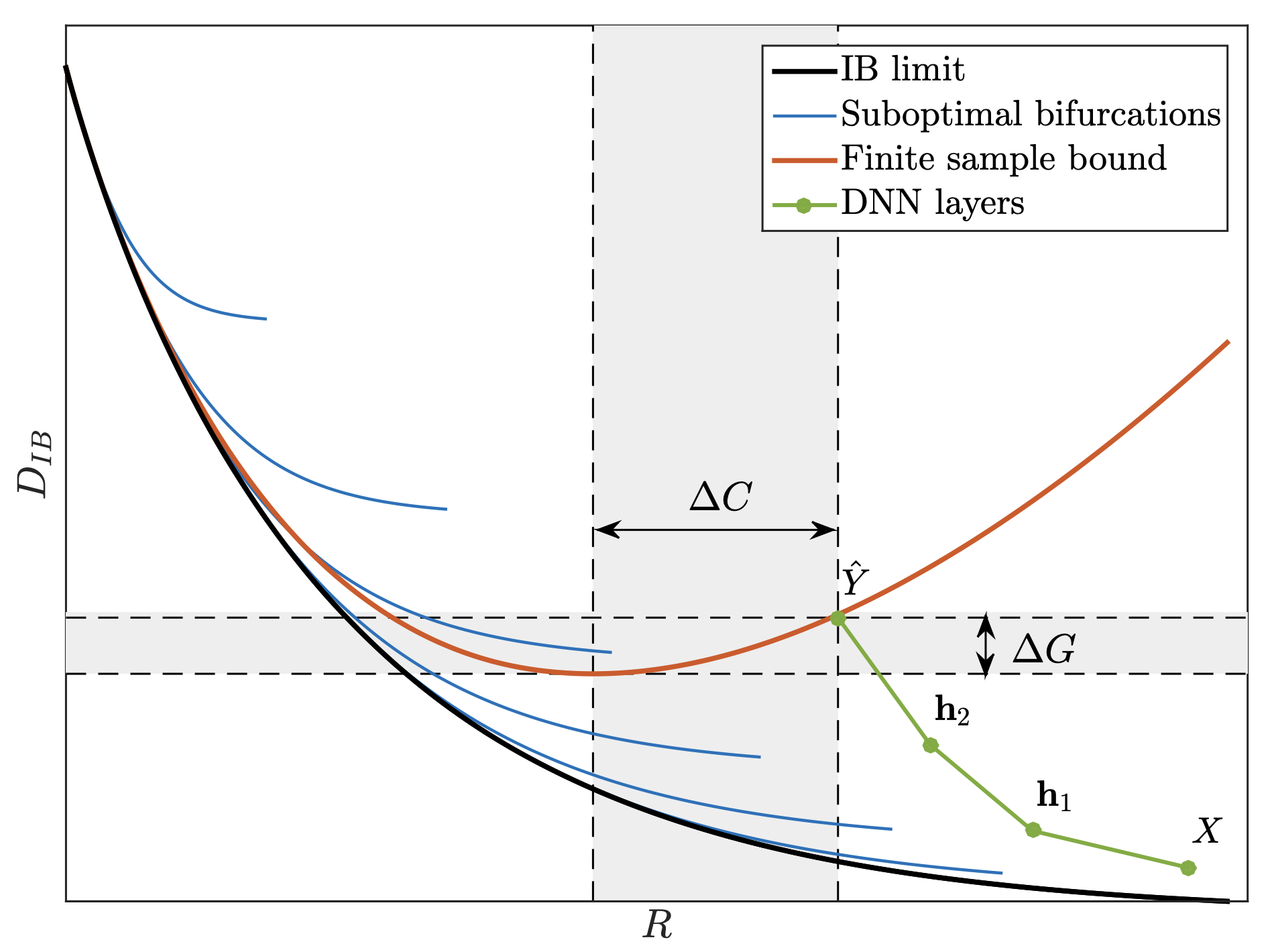
To say this in plain language, during training a deep network first learns to extract features that are informative about the label $Y$. This shows up as an increase in $I(T; Y)$ for a hidden layer $T$. In the same phase, $I(X; T)$ also increases, because the network is learning any feature at all. Then a second phase begins, where the network discards information about $X$ that is not useful for predicting $Y$. This shows up as $I(X; T)$ decreasing while $I(T; Y)$ stays high. The claim was backed by experiments on a small tanh network on a synthetic binary classification task, and the figure above is the picture that stuck.
Saxe et al. look at the activation function
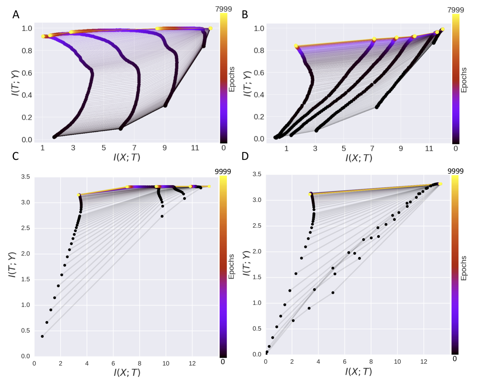
Saxe and collaborators redid the experiments with ReLU networks instead of tanh ones, and the compression phase simply did not appear. $I(X; T)$ did not decrease over training time. The compression that showed up for tanh was not a property of deep learning in general; it was a property of a saturating nonlinearity plus a binning-based mutual information estimator. Tanh units saturate, which effectively quantizes the hidden representation onto a finite set of states, and mutual information estimated by binning is extremely sensitive to quantization.
This was a serious blow. A lot of the theoretical appeal of the information bottleneck story came from the compression phase being read as a fundamental feature of deep learning. If it is an artifact of a particular activation measured with a particular estimator, the universal claim is gone.
Goldfeld et al. and the estimator problem
Goldfeld and collaborators formalized what Saxe et al. had noticed empirically. Mutual information for continuous random variables is not well-defined when the function from input to representation is deterministic. Writing it out, $I(X; T) = H(T) - H(T \mid X)$, and for a deterministic $T = f(X)$ the conditional entropy $H(T \mid X)$ is negative infinity, so $I(X; T)$ is infinity, always. The finite numbers everyone was plotting were artifacts of some combination of added noise, binning, and kernel-density estimators, and different choices gave different answers. The information-plane plots were therefore measuring a property of the measurement at least as much as a property of the network.
That is not a fatal blow, because you can define a noisy version of the network that does have well-defined mutual information, and study that. Goldfeld et al. do this carefully. But once you do, the specific two-phase trajectory is not robust across estimator choices, and the strong empirical support for the original claim evaporates.
What I think survives
A weaker claim survives the pushback comfortably. Deep networks trained with stochastic gradient methods tend to learn representations that are sufficient for the label and insensitive to irrelevant variations in the input. This is documented in many ways across many papers. Calling it “information bottleneck” is fine as a descriptive name. The stronger claim, that training is literally organized as a phase transition in mutual information, is not supported by careful measurement, and the even stronger claim that SGD is implicitly doing variational inference on the information bottleneck objective was never cleanly established.
What the paper did, and what I think is the reason it remains worth reading, is that it proposed a third lens on generalization in deep learning at a time when the field was dominated by two. Capacity-based lenses, VC and Rademacher, say generalization depends on how restrictive the hypothesis class is. Geometry-based lenses, flat versus sharp minima, say generalization depends on the shape of the loss landscape at the found solution. Tishby added a third, sufficient-statistics lenses, and that framing has turned out to be productive even where the specific empirical claim did not hold. (The InfoNCE objective [6] used in modern self-supervised learning is an information bottleneck relative in everything but name.)
Sometimes a wrong paper is more useful than a right one because it gives the field a vocabulary it did not have.
References
- [1] N. Tishby and N. Zaslavsky. Deep learning and the information bottleneck principle. arxiv 1503.02406, 2015.
- [2] R. Shwartz-Ziv and N. Tishby. Opening the black box of deep neural networks via information. arxiv 1703.00810, 2017.
- [3] A. M. Saxe, Y. Bansal, J. Dapello, M. Advani, A. Kolchinsky, B. D. Tracey, and D. D. Cox. On the information bottleneck theory of deep learning. ICLR, 2018.
- [4] Z. Goldfeld, E. van den Berg, K. Greenewald, I. Melnyk, N. Nguyen, B. Kingsbury, and Y. Polyanskiy. Estimating information flow in deep neural networks. arxiv 1810.05728, 2019.
- [5] A. A. Alemi, I. Fischer, J. V. Dillon, and K. Murphy. Deep variational information bottleneck. arxiv 1612.00410, 2017.
- [6] A. van den Oord, Y. Li, and O. Vinyals. Representation learning with contrastive predictive coding. arxiv 1807.03748, 2018.