Scaling laws from Kaplan to Chinchilla to broken laws, and what survives
Scaling laws tell us how much loss we will have. Everything else about the model, the interesting everything, is underdetermined by the loss number.
Key terms used in this post
- compute-optimal
- the allocation of a fixed compute budget to model size and dataset size that minimizes final loss.
- isoflops
- curves that hold compute fixed while varying model size; the minima trace out the scaling law.
- broken scaling laws
- Caballero et al.’s claim that the loss-vs-compute curve has piecewise structure rather than a single power law.
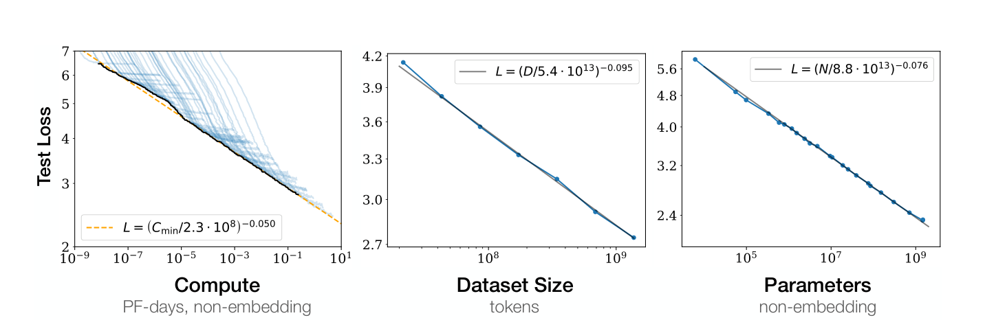
Kaplan et al. [1] published what became the reference point for thinking about how language model loss scales with compute, model size, and dataset size. The paper’s core claim is that test loss follows power-law decay in each of those variables, with clean exponents that fit over several orders of magnitude, and that for a fixed compute budget there is an optimal allocation between model size and data. That optimal allocation, the Kaplan paper argued, favors larger models over more data.
The result was consequential in a way most papers are not. Labs used it to plan training runs. The Chinchilla-scale models that came two years later existed in the shape they did partly because of what this paper said about how to spend compute. It is also, as it turned out, wrong about the specific allocation ratio in a way that changed the field again.
What Chinchilla found
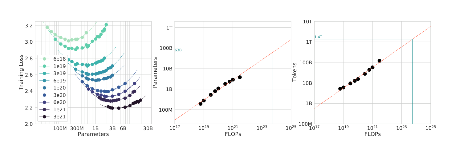
Hoffmann et al. [2] ran the question again at a much larger scale and with a much more careful experimental design. They trained over four hundred models spanning roughly four orders of magnitude in parameter count, at different compute budgets, and fit a joint surface to the resulting losses. The optimal ratio they found was not the Kaplan ratio. For every doubling of model size, we want to double the dataset size. Roughly twenty tokens per parameter at the optimum, as a rule of thumb that got quoted forever after.
This is a substantial correction to Kaplan, and Hoffmann argued the issue with the earlier paper was that its training runs were too short. Kaplan trained models to less than the compute-optimal point and extrapolated the trend line they were sitting on, rather than finding the actual minimum for each model size. When we do training runs long enough to reach a minimum, the minimum sits at a different model size than the extrapolation suggested.
The consequences of the correction
In hindsight, the practical lesson is that GPT-3 and its contemporaries were trained with too little data for their size. The Chinchilla paper showed that at their compute budget, a smaller model trained on more tokens would have had strictly lower loss. This is why Chinchilla-70B, despite being substantially smaller than the 175B GPT-3, outperformed it on most benchmarks. The model was Chinchilla-optimal at its compute budget; GPT-3 was Kaplan-optimal, which was the wrong target.
Everything downstream of this, the switch toward longer training runs, the data-scaling focus, the rise of smaller models trained longer, is calibrated against the Chinchilla target. Llama-2 trained seven billion parameters on two trillion tokens, which is well past Chinchilla-optimal and into the regime where we are trading compute-optimality for inference-time cost. The industry moved the target once more once people realized that serving a small model at inference is cheap and that the Chinchilla-optimal checkpoint is a training-cost optimum, not a deployment optimum.
Broken laws
Caballero et al. [3] argued that the power-law story is itself wrong. Their claim is that loss versus compute is not a smooth power law but a piecewise smooth function with a small number of inflection points and breaks. The power-law fits in Kaplan and Chinchilla are averaging across regimes that behave differently and producing a single exponent that corresponds to no regime in particular.
Whether the broken-laws framing is the right one depends on what we are using the fit for. For coarse extrapolation across orders of magnitude, the power law works. For fine-grained prediction of when a capability emerges at what scale, it does not, and the breaks that Caballero identifies correspond roughly to points where new capabilities start mattering for the loss. Emergent capabilities in the Wei et al. [4] sense, which Schaeffer et al. [5] later argued are an artifact of discretized metrics, are the same breaks from a different angle.
Gwern’s Scaling Hypothesis essay is the most thorough popular treatment of the underlying thesis that capabilities emerge from scale. It was written between Kaplan and Chinchilla, and its predictions about what additional scale would buy have held up surprisingly well. EpochAI has since taken on the empirical side, publishing replication, extrapolation, and broken-law analyses that sit downstream of both Kaplan and Chinchilla. Jacob Steinhardt’s Bounded Regret is the other blog that has thought carefully about what scaling laws do and do not let us forecast.
What survives
The predictive direction is robust across all three papers. Given a well-behaved architecture, a well-mixed dataset, and enough compute to be past the pretraining phase, we can extrapolate loss from smaller to larger runs and be approximately right. The error bars on the extrapolation grow with the distance, but not catastrophically. This is the single most useful thing the scaling laws literature gave us, and it is what labs use to decide whether to spend a billion dollars on a training run.
What does not survive is confidence in any specific exponent or ratio as universal. The exponent depends on architecture, data mixture, and the details of the optimizer. The Chinchilla ratio of twenty tokens per parameter is a point estimate for one particular setup; it moves with every change to the training recipe. The papers that extrapolated Kaplan’s ratio to plan multi-billion dollar training runs learned this the hard way, and the papers that are currently extrapolating Chinchilla’s ratio to plan the next round of runs will probably learn the same lesson in a couple of years.
What they never predicted
The scaling law literature is about test loss on the training distribution, and nothing else. It does not predict what data mixture to use, what architecture beats dense transformer, which capabilities emerge at what scale, whether model behavior is safe, or how training dynamics interact with the learning rate schedule. All of these are properties of the training run that live outside the scaling law fit. Treating the laws as if they settled any of these questions is the standard failure mode, and the broken-laws literature is largely an argument about how that failure mode shows up in specific predictions.
The honest statement is that scaling laws tell us how much loss we will have. Everything else about the model, the interesting everything, is underdetermined by the loss number. This is consistent with the loss number being very useful and also nowhere near sufficient.
References
- [1] J. Kaplan, S. McCandlish, T. Henighan, T. B. Brown, B. Chess, R. Child, S. Gray, A. Radford, J. Wu, and D. Amodei. Scaling laws for neural language models. arxiv 2001.08361, 2020.
- [2] J. Hoffmann et al. Training compute-optimal large language models. arxiv 2203.15556, 2022.
- [3] E. Caballero, K. Gupta, I. Rish, and D. Krueger. Broken neural scaling laws. arxiv 2210.14891, 2022.
- [4] J. Wei et al. Emergent abilities of large language models. arxiv 2206.07682, 2022.
- [5] R. Schaeffer, B. Miranda, and S. Koyejo. Are emergent abilities of large language models a mirage? arxiv 2304.15004, 2023.
- [6] T. Henighan et al. Scaling laws for autoregressive generative modeling. arxiv 2102.01293, 2021.
- [7] T. Pearce and J. Song. Reconciling Kaplan and Chinchilla scaling laws. arxiv 2406.12907, 2024.